wall-ctf (CATI) - Conduction Transfer Function Coefficients

Author: Valerio Lo Brano - Università degli Studi di Palermo

CATI computes the Conduction Transfer Function (CTF) coefficients for multilayer wall assemblies using the Z-transform method. This is the same mathematical approach used by TRNSYS, DOE-2, BLAST, TARP, and the ASHRAE Transfer Function Method (TFM) for dynamic thermal simulation of buildings.

The algorithm was originally developed as part of the Ph.D. dissertation of Valerio Lo Brano at the Università degli Studi di Palermo (Department of Energy and Environmental Research - DREAM), and later refined and published in two peer-reviewed journal articles (see How to cite). The original implementation (software THELDA / CATI2005, written in VB.NET) was used to simulate the thermal behaviour of massive historical buildings in the Mediterranean area, where the original Mitalas-Stephenson algorithm showed numerical limitations when applied to walls with high thermal inertia, typical of Southern European construction. The research led to the development of Procedure I (optimal pole and residue selection), which overcomes these limitations.

Given the thermophysical properties of a wall (layer thicknesses, densities, specific heats, conductivities), CATI determines the Z-domain transfer function coefficients that relate the heat flux at the internal surface to any generic input signal (external temperature, sol-air temperature, internal loads, etc.). Once computed, the coefficients are a property of the wall itself and can be reused for any input signal, any number of times, without recalculation. This is the key advantage of the method: the expensive computation is done once, and the subsequent simulations are extremely fast.

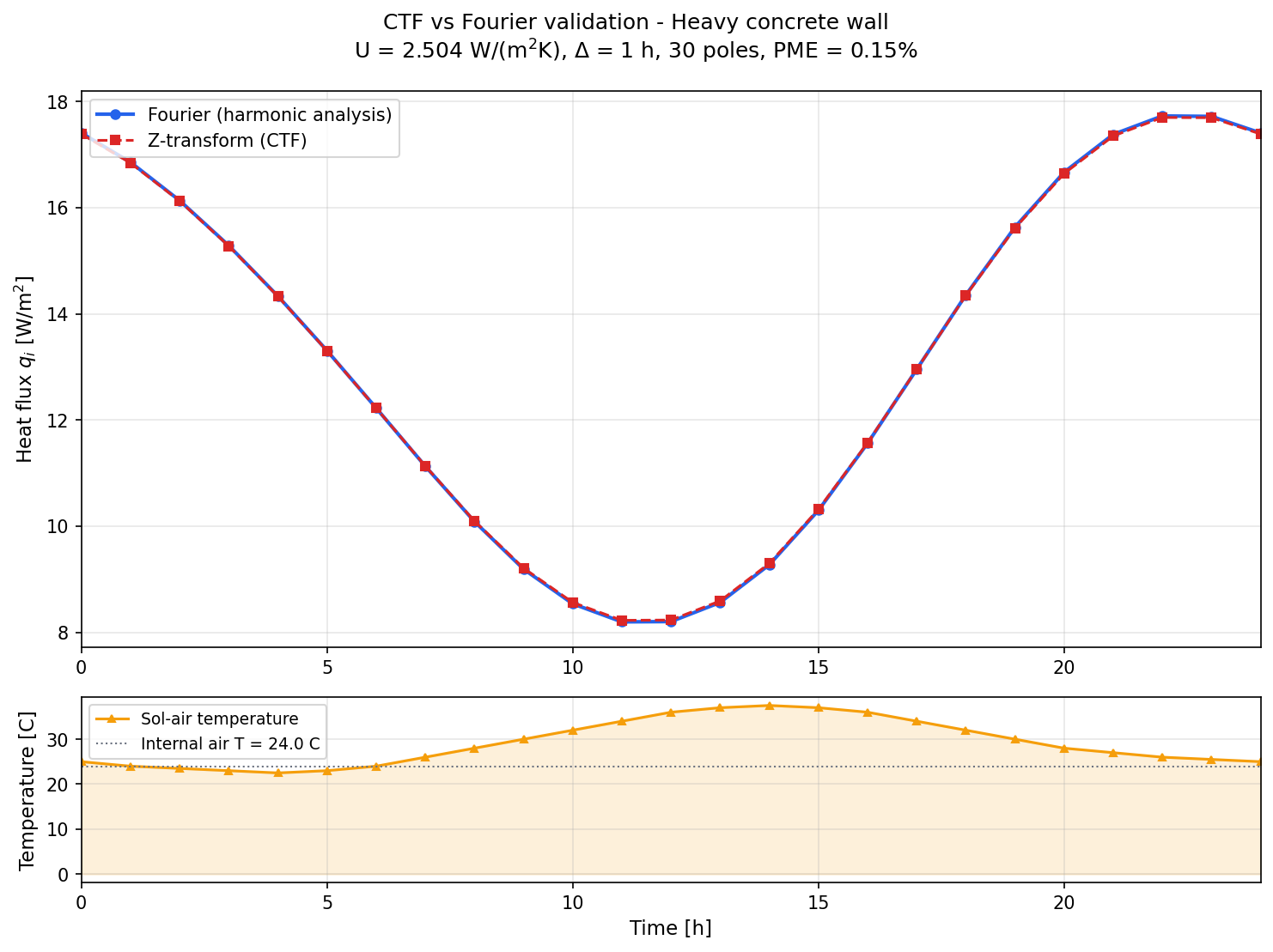
Validation example: comparison between the Z-transform (CTF) output and the independent Fourier (harmonic analysis) reference solution for a heavy concrete wall (plaster 2cm + concrete 25cm + plaster 2cm), subjected to a periodic temperature profile. The two curves are virtually indistinguishable (PME = 0.15%), confirming that the selected set of poles and residues accurately represents the wall's thermal dynamics. Once these coefficients are computed, they can be reused with any arbitrary input signal.

---

Table of contents

• Theoretical background
• Installation
• Quick start
• Input format
• Parameters and guidelines
• Examples
• Validation
• How to cite
• License

---

Theoretical background

Why the Laplace transform?

The thermal behaviour of a building wall is governed by the Fourier heat equation, a partial differential equation (PDE) that describes how temperature θ(x,t) and heat flux q(x,t) vary through a solid material over time:

$$\frac{\partial^2 \theta(x,t)}{\partial x^2} = \frac{1}{\alpha} \frac{\partial \theta(x,t)}{\partial t}$$

where α = λ / (ρ · Cp) is the thermal diffusivity.

Solving this PDE directly in the time domain is complex. The Laplace transform converts the problem from the time domain into the complex frequency domain (the s-domain), where the PDE becomes an ordinary differential equation that can be solved algebraically. The procedure, as described by Carslaw and Jaeger (1959), is:

1. Transform the time-domain equations into subsidiary equations in the complex s-domain
2. Solve the subsidiary equations by purely algebraic manipulation
3. Apply the inverse transform to return to the time domain

The thermal transmission matrix

In the Laplace domain, the relationship between temperature and heat flux on the two sides of a homogeneous isotropic layer of thickness L can be written in a compact matrix form:

$$\left\lbrace\begin{matrix} \theta(L,s) \\ q(L,s) \end{matrix}\right\rbrace = \left[\begin{matrix} a & b \\ c & d \end{matrix}\right] \times \left\lbrace\begin{matrix} \theta(0,s) \\ q(0,s) \end{matrix}\right\rbrace$$

where the elements of the transmission matrix M (whose determinant is unity) are:

$$a = d = \cosh\left(L\sqrt{\frac{s}{\alpha}}\right)$$

$$b = \frac{\sinh\left(L\sqrt{\frac{s}{\alpha}}\right)}{\lambda\sqrt{\frac{s}{\alpha}}}$$

$$c = \lambda\sqrt{\frac{s}{\alpha}} \cdot \sinh\left(L\sqrt{\frac{s}{\alpha}}\right)$$

with λ [W/(m K)] the thermal conductivity, ρ [kg/m³] the density, Cp [J/(kg K)] the specific heat, and α = λ/(ρ·Cp) [m²/s] the thermal diffusivity.

For surface resistance layers (convective + radiative films) and air gaps, the matrix is simply:

$$\left[\begin{matrix} 1 & R \\ 0 & 1 \end{matrix}\right]$$

where R is the thermal resistance.

For a multilayer wall composed of n layers, the overall transmission matrix is the ordered product of all individual layer matrices, from the external surface (x = 0) to the internal one (x = L):

$$\left[\begin{matrix} A(s) & B(s) \\ C(s) & D(s) \end{matrix}\right] = \left[\begin{matrix} a_1 & b_1 \\ c_1 & d_1 \end{matrix}\right] \times \left[\begin{matrix} a_2 & b_2 \\ c_2 & d_2 \end{matrix}\right] \times \cdots \times \left[\begin{matrix} a_n & b_n \\ c_n & d_n \end{matrix}\right]$$

where in general a = d for each single layer, but A ≠ D for the overall wall. By inverting this system, the heat fluxes on both surfaces can be expressed as functions of the two surface temperatures alone:

$$\left\lbrace\begin{matrix} q(0,s) \\ q(L,s) \end{matrix}\right\rbrace = \left[\begin{matrix} D/B & -1/B \\ 1/B & -A/B \end{matrix}\right] \times \left\lbrace\begin{matrix} \theta(0,s) \\ \theta(L,s) \end{matrix}\right\rbrace$$

This is the fundamental relation for the determination of the transfer functions, both in the time domain and in the frequency domain.

Why the Z-transform?

The Laplace-domain transfer function G(s) describes a continuous-time system, but building simulation works with discrete time steps (typically 1 hour), driven by sampled climatic data (hourly temperature, solar radiation, etc.). The Z-transform is the discrete-time counterpart of the Laplace transform: for a continuous function f(t) sampled at regular intervals Δ, its Z-transform is obtained by the substitution z = e^(sΔ):

$$f(0) + f(\Delta)z^{-1} + f(2\Delta)z^{-2} + \cdots$$

This converts the Laplace-domain transfer function into a ratio of polynomials in z⁻¹, which leads directly to a recursive formula computable at each time step, using only past values of inputs and outputs. This is extremely efficient for long simulations (e.g. a full year at hourly resolution = 8760 time steps).

From Laplace to Z-domain

From the inverted transmission matrix, the heat flux at the internal surface of a single wall in the Z-transform domain is (Ref. [1], Eq. 11):

$$Q_i(z) = \frac{1}{B(z)} \cdot T_e(z) - \frac{A(z)}{B(z)} \cdot T_i(z)$$

where the two sub-transfer functions 1/B and A/B link the heat flux respectively to the external (sol-air) and the internal air temperature.

Each sub-transfer function can be written as a ratio of two polynomials in z⁻¹:

$$G(z) = \frac{N(z)}{D(z)} = \frac{b_0 + b_1 z^{-1} + b_2 z^{-2} + \cdots + b_n z^{-n}}{1 + d_1 z^{-1} + d_2 z^{-2} + \cdots + d_n z^{-n}}$$

where N(z) (numerator) and D(z) (denominator) are in principle polynomials of infinite order, since the thermal system possesses infinitely many poles. In practice, the series is truncated to a finite number N of terms. The coefficients b_j and d_j are the CTF coefficients computed by CATI. The procedure to determine them is the following.

Step 1: Root finding

The poles sₙ of the system are the values of s that make DEN(s) = B(s) = 0. Since the poles must lie on the negative part of the real axis, the substitution √s = jδ is used, reducing the search to the real numbers domain (Ref. [1], Sec. 3).

Step 2: Heaviside partial-fraction expansion

Assuming a linear ramp as input signal, the Laplace-domain response is expanded as (Ref. [1], Eq. 4; Ref. [2], Eq. A.3):

$$O(s) = \frac{1}{s^2} G(s) = \frac{1}{s^2} \frac{\text{NUM}(s)}{\text{DEN}(s)} = \frac{C_0}{s^2} + \frac{C_1}{s} + \sum_{n=1}^{\infty} \frac{\text{res}_n}{s - s_n}$$

where C₀ and C₁ are the residuals linked to the double pole at the origin due to the ramp input, and resₙ are the residuals linked to the poles sₙ:

$$C_0 = \left[\frac{\text{NUM}(s)}{\text{DEN}(s)}\right]_{s=0}, \qquad \text{res}_n = \left[\frac{\text{NUM}(s)}{s^2 , \text{DEN}'(s)}\right]_{s=s_n}$$

The coefficient C₁ involves the derivatives DEN'(s) and NUM'(s) evaluated at s = 0 (Ref. [1], Sec. 3). In practice, the Mitalas instruction sets C₁ = −Σ resₙ to ensure the response starts at zero for t = 0.

The inverse Laplace transform returns the ramp response to the time domain:

$$O(t) = \mathcal{L}^{-1}\left[I(s) \cdot G(s)\right] = C_0 t + C_1 + \sum_{n=1}^{N} d_n , e^{\beta_n t}$$

where βₙ = sₙ < 0 are the poles (all on the negative real axis for a passive thermal system). Each term dₙ · e^(βₙt) is a decaying exponential that represents a thermal mode of the wall: poles close to zero correspond to slow modes (high thermal inertia), while poles far from zero correspond to fast modes that decay rapidly.

Step 3: Procedure I (optimal pole selection)

In theory, the thermal system has infinitely many poles. In practice, only a finite number N can be computed. Moreover, not all poles contribute significantly to the system response: the fast-decaying modes (large |βₙ|) have negligible effect after the first few time steps. Keeping too many poles, especially for massive walls, introduces numerical noise that can degrade the solution rather than improve it (Ref. [2], Sec. 4).

Procedure I (Ref. [2], Sec. 5) addresses this by sorting residues by absolute value in descending order |d̂₁| > |d̂₂| > ··· > |d̂ₙ| and retaining only the significant ones (|d̂ₙ| > σ, with σ = 10⁻¹⁰). The truncated transfer function:

$$\hat{G}(s) = \sum_{n=1}^{\hat{N}} \frac{\hat{d}_n}{s - \hat{p}_n}$$

captures the essential dynamics of the wall while avoiding the numerical problems that arise from insignificant poles.

Step 4: Z-domain transfer function

The Z-transform of the sampled ramp response gives (Ref. [1], Eq. 5-6; Ref. [2], Eq. A.6):

$$\frac{N(z)}{D(z)} = \frac{\dfrac{C_0 \Delta}{(1-z^{-1})^2} + \dfrac{C_1}{1-z^{-1}} + \displaystyle\sum_{n=1}^{N} \dfrac{\text{res}_n}{1-\mathrm{e}^{s_n \Delta} z^{-1}}}{\dfrac{C_0 \Delta}{z(1-z^{-1})}}$$

where Δ is the sampling period and the Z-domain denominator is:

$$D(z) = \prod_{n=1}^{N} \left(1 - \mathrm{e}^{s_n \Delta} , z^{-1}\right)$$

The numerator N(z) is a polynomial obtained from the convolution of the sampled ramp response with the second differences of the denominator coefficients (Ref. [1], Eq. 5).

Step 5: Recursive formula

Applying the definition of the TFM and expanding the terms (Ref. [2], Eq. A.7-A.8), the generic partial output at time nΔ is:

$$T_{x,i}(n\Delta) = \sum_{j=0}^{n} b_j \cdot I_i\left[(n-j)\Delta\right] - \sum_{j=1}^{n} d_j \cdot T_{x,i}\left[(n-j)\Delta\right]$$

For the specific case of the wall heat flux, with the external temperature T_e and the constant internal air temperature T_i as inputs:

$$q_i(n\Delta) = \sum_{j=0}^{n} b_j \cdot T_e\left[(n-j)\Delta\right] - \sum_{j=1}^{n} d_j \cdot q_i\left[(n-j)\Delta\right] - T_i \sum_{j=0}^{n} c_j$$

where b_j are the numerator coefficients of 1/B (external temperature contribution), c_j are the numerator coefficients of A/B (internal temperature contribution), and d_j are the common denominator coefficients.

This is a recursive formula: at each time step n, the output depends on the current and past input values and on the past output values. Once the coefficients b_j, c_j, d_j are known, the computation is extremely fast: a single wall requires only a few multiplications and additions per time step, regardless of the wall's complexity. This is the key advantage of the TFM over finite-difference or finite-element methods.

The global response of each inner surface temperature is obtained by superimposing all partial outputs from different inputs (Ref. [2], Eq. A.9):

$$T_x(n\Delta) = \sum_{i}^{\text{all inputs}} T_{x,i}(n\Delta)$$

Transfer function coefficients have to be calculated for each different pair of input-output (e.g. sol-air temperature, inner air temperature, inner thermal loads, etc.). All of the outputs referred to the same physical node are later summed to obtain the global response.

Procedure I: optimal pole selection

As demonstrated in Ref. [2], for massive building walls typical of the Mediterranean architectural heritage, a naive application of the TFM with many poles can produce worse results than using fewer poles. The Percentage Mean Error (PME) can increase from < 1% to > 1000% when using 15 poles instead of 5.

CATI implements Procedure I from Ref. [2]: residues are sorted by absolute value in descending order, and only those above a significance threshold (|resₙ| > 10⁻¹⁰) are retained. This guarantees PME < 1% for all standard wall constructions at 1-hour sampling period.

---

Installation

With uv (recommended)

uv is the fastest way to manage Python projects:

# Clone the repository
git clone https://github.com/valeriolobrano/wall-ctf.git
cd wall-ctf

# Install with uv (creates virtualenv automatically)
uv sync

# Run tests
uv run pytest

# Run the CLI
uv run cati examples/heavy_wall.json

# Run with optional plotting support
uv add matplotlib
uv run python scripts/generate_figures.py

With pip

pip install wall-ctf

Or from source:

git clone https://github.com/valeriolobrano/wall-ctf.git
cd wall-ctf
pip install .

# With plotting support
pip install ".[plot]"

Requirements

• Python >= 3.12
• NumPy >= 1.26
• matplotlib >= 3.8 (optional, for plotting)

---

Quick start

Basic example: single wall

from cati import Wall, Layer, compute_ctf

# Define a wall from outside to inside:
#   external surface resistance -> material layers -> internal surface resistance
# All values in SI units
wall = Wall(layers=[
    Layer(name="External surface", resistance=0.04),       # m2*K/W
    Layer(name="Concrete", thickness=0.25, density=2400,   # m, kg/m3
          specific_heat=1000, conductivity=1.4),           # J/(kg*K), W/(m*K)
    Layer(name="Internal surface", resistance=0.13),
])

result = compute_ctf(wall, n_roots=30, n_coefficients=20)

print(f"U-value: {result.thermal_transmittance:.3f} W/(m2*K)")
print(f"Significant poles: {result.n_poles}")
print(f"Effective coefficients: {result.n_coefficients}")

With Fourier validation (quality check)

import numpy as np

# 24-hour periodic temperature profile for validation (hourly, 25 values with wrap-around)
# This can be any signal: sol-air temperature, outdoor air temperature, etc.
profile = np.array([
    25.0, 24.0, 23.5, 23.0, 22.5, 23.0,   # 0h-5h
    24.0, 26.0, 28.0, 30.0, 32.0, 34.0,   # 6h-11h
    36.0, 37.0, 37.5, 37.0, 36.0, 34.0,   # 12h-17h
    32.0, 30.0, 28.0, 27.0, 26.0, 25.5,   # 18h-23h
    25.0,                                   # 24h = 0h
])

result = compute_ctf(
    wall,
    n_roots=30,
    n_coefficients=20,
    temperature_profile=profile,
    T_int=24.0,              # constant internal temperature [C]
    sampling_time=1.0,       # sampling period [hours]
    n_periods=20,            # periods to exit transient
    validate_fourier=True,   # compare with harmonic solution
)

print(f"Fourier validation error: {result.fourier_error:.2f}%")
# Output: Fourier validation error: 0.15%
# A low error confirms the CTF coefficients are accurate for this wall.
# These coefficients can now be reused with ANY input signal.

Using the CTF coefficients in a simulation

nc = result.n_coefficients  # number of effective coefficients
b = result.b_coeffs[:nc+1]  # numerator for external temperature
c = result.c_coeffs[:nc+1]  # numerator for internal temperature
d = result.d_coeffs[:nc+1]  # denominator (common)

# Simulation loop (hourly time step)
T_int = 24.0
q = np.zeros(8760)  # one year, hourly

for n in range(1, 8760):
    # b * T_external (convolution)
    q[n] = sum(b[j] * T_ext_hourly[max(0, n-j)] for j in range(nc+1))
    # - d * q_past (recursive feedback)
    q[n] -= sum(d[j] * q[max(0, n-j)] for j in range(1, nc+1))
    # - c * T_internal (constant offset)
    q[n] -= T_int * sum(c)

Parallel computation for multiple walls

from cati import compute_ctf_batch

# Compute CTF for all walls of a building in parallel
walls = [wall_north, wall_south, wall_east, wall_west, roof, floor]
results = compute_ctf_batch(walls, n_roots=30, n_coefficients=20)

for wall, result in zip(walls, results):
    print(f"{wall.name}: U={result.thermal_transmittance:.3f}, "
          f"poles={result.n_poles}, coeffs={result.n_coefficients}")

Command-line interface

# Compute and print CTF coefficients as JSON
uv run cati examples/heavy_wall.json --roots 30 --coefficients 20

# Save results to file
uv run cati examples/heavy_wall.json -o results.json

# Custom parameters
uv run cati wall.json --sampling-time 2 --periods 30 --t-int 26

# Skip Fourier validation (faster)
uv run cati wall.json --no-fourier

Loading walls from JSON

from cati import Wall

# From a JSON file
wall = Wall.from_json("examples/heavy_wall.json")

# From a Python dictionary
wall = Wall.from_dict({
    "name": "My wall",
    "layers": [
        {"name": "Ext", "resistance": 0.04},
        {"name": "Brick", "thickness": 0.12, "density": 1700,
         "specific_heat": 800, "conductivity": 0.84},
        {"name": "Int", "resistance": 0.13},
    ]
})

---

Input format

JSON wall definition

{
    "name": "Concrete wall with plaster",
    "layers": [
        {"name": "External surface", "thickness": 0.0, "resistance": 0.04},
        {"name": "External plaster", "thickness": 0.02, "density": 1800,
         "specific_heat": 1000, "conductivity": 0.9},
        {"name": "Concrete block", "thickness": 0.25, "density": 2400,
         "specific_heat": 1000, "conductivity": 1.4},
        {"name": "Internal plaster", "thickness": 0.02, "density": 1400,
         "specific_heat": 1000, "conductivity": 0.7},
        {"name": "Internal surface", "thickness": 0.0, "resistance": 0.13}
    ],
    "temperature_profile": [25, 24, 23.5, 23, 22.5, 23, 24, 26, 28, 30,
                            32, 34, 36, 37, 37.5, 37, 36, 34, 32, 30,
                            28, 27, 26, 25.5]
}

Units (SI)

Property	Unit	Description
thickness	m	Layer thickness (0 for surface resistance or air gap)
density	kg/m^3	Material density
specific_heat	J/(kg*K)	Specific heat capacity
conductivity	W/(m*K)	Thermal conductivity
resistance	m^2*K/W	Thermal resistance (for air gaps and surface films)

Wall structure rules

A wall must contain at least 3 layers:

1. First layer: external surface resistance (combined convective and radiative exchange coefficient)
2. Intermediate layers: material layers or air gaps, ordered from outside to inside
3. Last layer: internal surface resistance

Typical surface resistance values (EN ISO 6946):

Surface	Resistance [m^2*K/W]	Notes
External, normal exposure	0.04	Wind speed > 4 m/s
External, sheltered	0.06	Wind speed 1-4 m/s
Internal, horizontal flow	0.13	Vertical walls
Internal, upward flow	0.10	Floors (heating)
Internal, downward flow	0.17	Ceilings (heating)

---

Parameters and guidelines

Parameter	Default	Description
n_roots	50	Number of zeros of B(s) to find
n_coefficients	49	Maximum number of Z-domain coefficients
sampling_time	1.0	Sampling period [hours] (must divide 24)
n_periods	10	Number of 24h periods for transient decay
n_harmonics	120	Harmonics for Fourier validation
T_int	24.0	Constant internal air temperature [C]
use_mitalas	True	Apply Mitalas instruction (recommended)

Recommendations

Based on the analysis in Ref. [2]:

1. Do not use too many poles. For most walls, 20-30 roots with automatic Procedure I selection gives optimal results. The effective number of poles is determined automatically.

2. Increase the sampling period for massive walls. For walls with total thickness > 0.4 m (typical of historical European buildings), a sampling period of 2 h may give better results than 1 h.

3. Procedure I is enabled by default. It sorts residues by significance and discards negligible ones, preventing the numerical problems that affect naive implementations.

4. Check the Fourier validation error. A PME below 5% indicates reliable coefficients. If the error is high, try:

   • Increasing the sampling period
   • Reducing n_roots
   • Checking wall data for unrealistic property values

---

Examples

The examples/ directory contains ready-to-use JSON wall definitions:

• heavy_wall.json: Plaster + concrete 25cm + plaster (U = 2.50 W/m^2K)
• insulated_wall.json: Insulated cavity wall with air gap (U = 0.33 W/m^2K)

Run them with:

uv run cati examples/heavy_wall.json --roots 30 --coefficients 20

---

Validation

The purpose of the Fourier comparison is not to provide an alternative simulation method, but to verify whether the finite set of poles and residues selected by CATI is a good approximation of the wall's exact (infinite-order) transfer function. The Fourier (harmonic) solution uses the complex thermal quadrupole to compute the exact periodic steady-state response for a given input signal. Since this approach operates in the frequency domain, it must be recomputed entirely for every different input signal, making it unsuitable for general-purpose simulation. On the contrary, the CTF coefficients are computed once and reused for any input.

The Percentage Mean Error (PME) between the CTF output and the Fourier reference is computed as in Ref. [2], Eq. (4-5):

$$\text{PME} = \frac{1}{24} \sum_{\tau=1}^{24} \frac{\left| T_Z(\tau) - T_F(\tau) \right|}{\left| T_F(\tau) \right|} \times 100$$

A low PME confirms that the truncated set of poles/residues faithfully represents the wall's thermal dynamics. Typical results:

Wall type	Thickness	U [W/m^2K]	PME
Heavy concrete + plaster	0.29 m	2.50	0.15%
Brick + concrete (2 layers)	0.27 m	~2.5	< 5%
Lightweight wood	0.10 m	1.20	~5%

---

How to cite

If you use CATI in your research, please cite the following publications:

G. Beccali, M. Cellura, V. Lo Brano, A. Orioli, "Single thermal zone balance solved by Transfer Function Method", Energy and Buildings 37 (2005) 1268-1277. DOI: 10.1016/j.enbuild.2005.02.010

G. Beccali, M. Cellura, V. Lo Brano, A. Orioli, "Is the transfer function method reliable in a European building context? A theoretical analysis and a case study in the south of Italy", Applied Thermal Engineering 25 (2005) 341-357. DOI: 10.1016/j.applthermaleng.2004.06.010

BibTeX entries are available in the CITATION.cff file.

---

License

GPL-3.0-or-later (GNU General Public License v3 or later)

• Free for academic, educational, and any use, including commercial.
• Copyleft: any derivative work must be distributed under the same GPL license and must release its source code.
• Citation required (Section 7b): any use must cite the publications listed above.
• Commercial licensing without GPL obligations is available upon request. Contact: valerio.lobrano@unipa.it

Copyright (c) 2005-2026 Valerio Lo Brano, Università degli Studi di Palermo.

See LICENSE for the full license text.