PINNStudio

A no-code desktop GUI for building, training, and visualizing Physics-Informed Neural Networks (PINNs) — built on DeepXDE.

One PDE, three dimensions — the same panel drives all of them, solved and visualized entirely within PINNStudio.

1D — (x, t) — Burgers

2D — (x, y, t) — Allen-Cahn (Wight & Zhao)

3D — (x, y, z, t) — Heat

Website  ·  Quick Start  ·  Templates  ·  Your Own PDE  ·  Discussions  ·  Citation

Table of contents

• Quick Install
• Overview
• Demo Video
• Features
• Repository Structure
• Quick Start
• Running PINNStudio Again
• What Gets Installed
• Built-in Templates
• Getting Started with Your Own PDE
• How It Works
• Citation
• References
• Acknowledgment
• Contributing
• Contact
• License

---

Quick Install

The fastest way to try PINNStudio (any OS, no GPU-driver matching):

pip install pinnstudio
pinnstudio

Have an NVIDIA GPU? Use the full install script instead - it detects your GPU and automatically installs a matching PyTorch build for you, which the plain pip install above does not do. See Quick Start below.

Command not found after pip install?

• pip: command not found? Use pip3 instead - many systems (macOS especially) only ship pip3, not a plain pip.
• pinnstudio: command not found even though the install said it succeeded? pip installed it into a per-user folder that is not on your shell's PATH yet. The install output actually tells you the exact folder, in a line like WARNING: The script pinnstudio is installed in '.../bin' which is not on PATH. Add that folder to your PATH:

echo 'export PATH="<folder from the warning above>:$PATH"' >> ~/.zshrc
source ~/.zshrc

(Use /.bashrc instead of /.zshrc if your shell is bash.) Then pinnstudio should launch directly. This never comes up with install.sh/install.bat, since those use a virtual environment where the command is always found automatically.

• The suggested GPU fix command itself fails with a flit_core or "Could not find a version that satisfies" error? Your pip is too old to resolve PyTorch's package index correctly. Upgrade it first, then retry:

python -m pip install --upgrade pip
pip install torch --index-url https://download.pytorch.org/whl/cu121 --force-reinstall

---

Overview

Setting up a Physics-Informed Neural Network usually means writing a new DeepXDE script for every problem: defining the PDE residual, wiring up boundary and initial conditions, picking collocation points, choosing an optimizer schedule, and writing your own plotting/error-analysis code afterward.

PINNStudio replaces that boilerplate with a form. You describe the problem — the PDE, the domain, the boundary and initial conditions, the network architecture, the training schedule — through the interface, and PINNStudio generates a standalone DeepXDE/PyTorch script, runs it, and streams the training log, loss curves, and solution plots back into the GUI.

It supports both forward problems (solve a known PDE) and inverse problems (estimate unknown PDE parameters from observation data), across 1D (x, t), 2D (x, y, t), and 3D (x, y, z, t), including coupled, multi-output PDE systems. The domain itself isn't limited to a box either — 2D problems can be posed on a rectangle, disk, ellipse, triangle, or arbitrary polygon, and 3D problems on a cuboid or sphere, so a re-entrant-corner or curved-boundary problem doesn't need any code of your own to set up.

The goal is to make physics-informed machine learning accessible to researchers who need it but don't want to become deep learning engineers first. Setting up a PINN by hand touches autograd-based residuals, collocation sampling, loss weighting, and optimizer scheduling all at once — details that are easy to get subtly wrong and can cost hours of debugging before a single result can be trusted. PINNStudio lets researchers across science and engineering — materials science, mechanics, chemistry, biology, and beyond — set up and run both forward and inverse PINN problems for their own equations without building that infrastructure from scratch, on a framework that has been thoroughly tested so results are trustworthy from the first run.

Demo Video

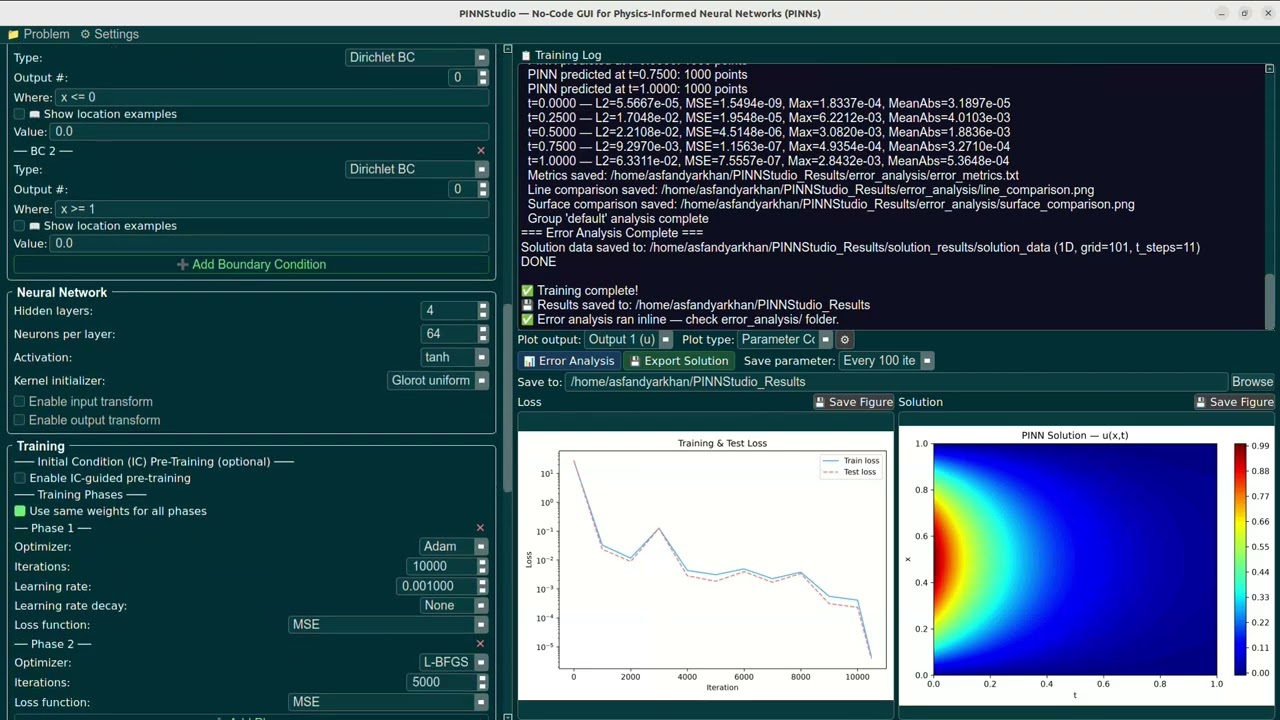
Click to watch a full walkthrough of the PDE setup panel on YouTube.

Features

Problem Setup

1D, 2D, and 3D problem definitions

Every problem is defined over (x, t), (x, y, t), or (x, y, z, t) — switching dimension in the Setup panel rebuilds the relevant controls (geometry selector, boundary condition rows, plot options) for you, so nothing from a previous dimension is left over and silently wrong. Steady-state (time-independent) problems are supported in every dimension too — turn off the time axis and the network trains a pure u(x), u(x, y), or u(x, y, z) instead.

Forward and inverse problems

Forward: the PDE's parameters are known — PINNStudio solves for the field itself. Inverse: one or more PDE parameters are unknown, and PINNStudio estimates them from observation data (a reference solution file) while solving for the field simultaneously. Every built-in template supports both modes; switching to Inverse auto-loads that template's own end-time reference file as the observed-data source and defaults its loss weight to 100, so estimating a parameter needs no manual file browsing to get started (still fully overridable). Multiple unknown parameters in the same problem are supported, not just one.

Free-form, multi-output PDE editor

Write the PDE residual directly as an expression, not through a fixed set of presets. Derivatives use a plain d<output>_<vars> naming convention — du_x, du_xx, du_t, du_xy, du_xt, all the way up to mixed fourth-order terms like du_xxyy or du_xxtt — so anything from a first-order diffusion term to a coupled, higher-order system is expressible without touching any generated code. Multi-output, coupled PDE systems (naming a second output v gives you dv_x, dv_t, and so on, alongside u's own) are supported the same way — the 2D Burgers and 1D Schrödinger templates below are both two-output coupled systems set up entirely through this editor.

Boundary and initial conditions

Boundary conditions are added as rows in a panel, each with its own type (Dirichlet, Neumann, Robin, Periodic, Point Set from a data file, or an advanced Operator/Interface condition), the output it applies to, and a True/False location expression in x, y, z that picks out which boundary it means (e.g. x >= 1) — compared against your own domain bounds, not a hardcoded number, so the same row still makes sense if you change the domain later. Initial conditions are set from an expression in x (y, z too in 2D/3D) or loaded from a data file, per output.

Geometry & domains

2D problems aren't limited to a rectangle: Rectangle, Disk, Ellipse, Triangle, and arbitrary Polygon (given as a vertex list) are all selectable geometries, each with its own domain-preview and parameter panel. 3D problems support Cuboid and Sphere. Picking a non-box shape doesn't change how you write BCs — the same location-expression convention still works, since DeepXDE only ever evaluates it on points already confirmed to be on that shape's boundary.

Collocation point controls

Domain, boundary, initial, and test point counts are all independently configurable, along with the sampling distribution, plus a live domain preview — a real, non-uniform PDE-collocation point cloud (domain points, boundary points, and initial-condition points, color-coded) plotted directly against your actual geometry, alongside a second panel showing the same points' distribution over time — so you can see exactly what will be handed to training before you click Solve. This works in 2D against any of the five 2D shapes (Rectangle, Disk, Ellipse, Triangle, Polygon) and in 3D too, with a real 3D scatter plot against a Cuboid or Sphere outline, not just a flat 2D preview.

2D preview — Rectangle

2D preview — Disk

3D preview — Cuboid

Training

Configurable network architecture

Hidden layer count, neurons per layer, activation function (tanh, ReLU, sigmoid, swish), and kernel initializer (Glorot uniform, Glorot normal, He uniform, He normal, zeros) are all exposed directly — no need to edit a script to try a wider or deeper network, a different nonlinearity, or a different weight initialization.

Input/output scaling

Optional affine rescaling on the way into and out of the network — $x_{\text{transformed}} = x_{\text{raw}} \times \text{scale} + \text{shift}$ per input dimension, and the same for each output — off by default (scale = 1, shift = 0 is the identity). Useful when a problem's natural coordinate or solution range is far from the network's comfortable operating range (e.g. a domain spanning thousands of units, or a solution that's always around $10^{-6}$) and normalizing it improves training behavior.

Two-stage optimization (Adam + L-BFGS)

Every run trains with Adam first, then hands off to L-BFGS for the second stage — a standard, effective PINN training recipe — with L-BFGS's own convergence settings exposed, and a configurable float precision (float32 for speed, float64 when L-BFGS needs the extra precision to converge cleanly).

Multi-phase optimizer scheduling and IC-guided pre-training

Beyond the basic two-stage recipe, training can be broken into any number of phases (different optimizers, iteration counts, and loss weights per phase), and an optional IC-guided pre-training pass can warm-start the network toward the initial condition before the full PDE-residual loss is even switched on — useful for problems where a cold-start network otherwise struggles to find the right basin.

Residual-based Adaptive Refinement (RAR)

Periodically resamples collocation points toward wherever the PDE residual is currently largest, concentrating training effort on the hardest parts of the domain (a sharp front, a boundary layer) instead of spreading points uniformly the whole time. Supported in every dimension.

Time-Adaptive training

Splits the time domain into a sequence of step groups and trains through them in order, optionally with transfer learning so each step warm-starts from the previous one's converged weights instead of training from scratch — effective for problems with a wide time window or fast-evolving dynamics that a single training pass struggles to fit all at once (see the two 2D Allen-Cahn templates below, both wide time windows that ship with Time-Adaptive on by default for exactly this reason). It works in 1D, 2D, and 3D alike.

One setting is worth understanding before using it in 3D: the "IC grid resolution" control is a per-axis point count for the grid handed between steps — 1D uses it directly, 2D squares it, and 3D cubes it, so a value that's perfectly reasonable in 1D/2D (101, say — 101² ≈ 10,201 points in 2D) becomes over a million points per step in 3D. PINNStudio defaults this to a 3D-safe value automatically when you switch into 3D, and shows an in-panel warning if you manually pick a larger one anyway — both added after exactly this scenario ran a real GPU out of memory partway through a 3D run.

Training callbacks — early stopping, checkpointing, time budget

Three optional, independently configurable callbacks, alongside Point Resampling (RAR, described above): Early Stopping halts training once the monitored loss (training or testing) stops improving by more than a minimum delta for a set number of iterations, with an optional baseline loss and a minimum iteration count before it can trigger. Model Checkpoint periodically saves the model during training — on a fixed iteration interval, either unconditionally or only when the monitored loss improves — which is also what makes a run resumable later through Restore & Visualize. Training Timer stops training after a wall-clock time budget (in minutes) regardless of iteration count, useful for a shared or time-limited machine.

Note: an earlier version of PINNStudio had a separate "Mini-batch training" option. It's gone — DeepXDE's PDE/TimePDE data classes ignore the batch_size argument entirely for this training pattern, so it was a no-op that changed nothing. Point Resampling (RAR) is the actual mechanism DeepXDE recommends in its place, and PINNStudio already implements it.

Live parameter convergence (Inverse mode)

For an inverse problem, the estimated parameter's value is logged and saved periodically throughout training — including during the L-BFGS phase, not just once at the very end — so you can watch it converge (or fail to) as training progresses, and plot its convergence history afterward as a static figure or an animated GIF. When the parameter's true value is known (every built-in template's Inverse setup, or one you supply yourself), both the plot and the GIF draw it as a dashed reference line alongside the run's own final estimate — including when you revisit an older run through Restore & Visualize's Parameter Convergence Plot/Animation, which reads the true value back from that run's saved model_config.json, or lets you type one in directly.

Analysis & Output

Live training log

Training runs as a background process with its stdout streamed straight into the Training Log panel in real time, with a Stop control that actually terminates the running process rather than just detaching from it.

Error analysis against reference data

Point a run at one or more reference solution files (at one or more time snapshots) and PINNStudio reports, for predicted values $u_{\text{pred}}$ against ground truth $u_{\text{true}}$ over $N$ evaluation points:

$$\Large L_2 \text{ relative error} = \frac{\lVert u_{\text{pred}} - u_{\text{true}} \rVert_2}{\lVert u_{\text{true}} \rVert_2}, \qquad \text{MSE} = \frac{1}{N}\sum_{i=1}^{N}\left(u_{\text{pred},i} - u_{\text{true},i}\right)^2$$

$$\Large \text{Max error} = \max_i \left| u_{\text{pred},i} - u_{\text{true},i} \right|, \qquad \text{Mean absolute error} = \frac{1}{N}\sum_{i=1}^{N}\left| u_{\text{pred},i} - u_{\text{true},i} \right|$$

alongside line-comparison and surface-comparison plots of the PINN prediction against ground truth. All twelve built-in templates ship with bundled reference data so this works immediately with no setup; it works the same way for a data file of your own.

Configurable result plotting

Static Surface or Line plots, or animated GIFs of either over time, with colormap, contour resolution, DPI, colorbar, and snapshot-count all configurable. For a 1D time-dependent Surface plot (static or animated), the two axes can be swapped between "x on the x-axis, t on the y-axis" and the reverse — whichever reads more naturally for your problem.

Solution data export

The raw predicted solution — not just the rendered plot — is saved alongside the run's other output, so it's available for your own downstream analysis outside the GUI.

Export as a standalone DeepXDE script

Every configured problem can be exported as a clean, dependency-minimal DeepXDE/PyTorch script (File → Export as DeepXDE Script...) — the same script the GUI itself would run, but meant to be read and handed off: to a cluster job, a collaborator without PINNStudio installed, or as a starting point for a hand-written project.

Restore & Visualize

Reload a saved checkpoint — no retraining needed

Point the Restore panel at a saved model checkpoint and its model_config.json, and PINNStudio reloads the trained network and regenerates whichever visualization you ask for — a static Surface or Line plot, an animated GIF of either, or (for a saved Inverse run) the parameter convergence history — without retraining anything. An animated result plays directly in the panel, the same as it would right after a fresh Solve, and Error Analysis re-runs against the same reference data if it was configured for that run originally.

Repository Structure

pinnstudio/
├── pinnstudio/
│   ├── main.py            # Entry point
│   ├── ui/
│   │   └── main_window.py # PyQt6 interface — every tab, dialog, and control
│   └── core/
│       ├── config.py      # PINNConfig — the full problem definition
│       ├── codegen.py     # PINNConfig -> standalone DeepXDE/PyTorch script
│       └── runner.py      # Runs the generated script, streams output to the GUI
├── assets/
│   ├── screenshots/        # README screenshots
│   └── results/             # Example output (solution images, demo GIFs)
├── reference_data/          # Bundled ground truth for the built-in templates
│   ├── 1D/
│   ├── 2D/
│   └── 3D/
├── requirements.txt
├── setup.py
├── install.sh              # One-command setup (macOS/Linux)
├── install.bat              # One-command setup (Windows)
└── README.md

Quick Start

Step 1: Open a terminal

• Windows: click the Start menu, type PowerShell, and open Windows PowerShell.
• macOS: press Cmd + Space to open Spotlight, type Terminal, and press Enter (or find it under Applications -> Utilities -> Terminal).
• Linux: open your terminal application (commonly Ctrl + Alt + T, or search "Terminal" in your application menu).

Step 2: Check you have git and Python 3.9+

Paste these one at a time:

git --version
python3 --version

(On Windows, use python --version instead of python3 --version.)

If either command isn't recognized:

• git missing? Install it from git-scm.com/downloads. Default options are fine. On macOS, running git --version for the first time may itself prompt you to install Apple's Command Line Tools — accept and let it finish, then try again.
• Python missing, or older than 3.9? Install it from python.org/downloads. On Windows, check "Add python.exe to PATH" on the installer's first screen — this is the single most common thing people miss.

After installing either one, close your terminal window completely and open a new one before continuing, so the change takes effect.

Step 3: Clone and install

git clone https://github.com/AsfandyarKhan72/PINNStudio.git
cd PINNStudio

macOS / Linux:

bash install.sh
./venv/bin/pinnstudio

Windows:

install.bat
.\venv\Scripts\pinnstudio.exe

The install script creates an isolated virtual environment inside the PINNStudio folder and installs PINNStudio and its dependencies into it — nothing is installed system-wide, and deleting the folder removes it completely. If it detects an NVIDIA GPU that the default PyTorch build can't use (an older driver, most commonly), it automatically installs a more compatible PyTorch build instead, so GPU support works out of the box on more machines. This step needs an internet connection and can take a few minutes.

Already have a working PyTorch + CUDA setup, or no GPU at all? You can also install with pip install pinnstudio - just be aware it skips the GPU compatibility check above, so if you hit a GPU-related error afterward, re-run install.sh / install.bat instead.

Step 4: Take the 60-second tour

Maximize the window for the best view — PINNStudio packs a lot of controls into the left panel. With the app open, leave the dimension on 1D, pick 1D Heat from the Quick Examples dropdown, and click Solve. The Training Log panel will stream progress, and the loss/solution plots will populate once the run finishes.

Something not working?

Open an issue on GitHub with the exact command you ran and the full error message — see Contributing.

Running PINNStudio Again

You only need to run the install steps above once. After that, launch PINNStudio again anytime with:

macOS / Linux, from inside the PINNStudio folder:

./venv/bin/pinnstudio

Windows, from inside the PINNStudio folder:

.\venv\Scripts\pinnstudio.exe

That's it - no need to reinstall or recreate the virtual environment.

What Gets Installed

install.sh / install.bat (used in Quick Start above) set up an isolated Python virtual environment and install:

• DeepXDE (PyTorch backend)
• PyTorch
• PyQt6
• NumPy
• Matplotlib
• Pandas

A CUDA-capable GPU is optional but recommended for larger 2D/3D problems and inverse runs.

Built-in Templates

Each template preconfigures the PDE, domain, boundary/initial conditions, network size, and training schedule — pick one from Quick Examples, then adjust as needed. All twelve support both Forward and Inverse mode.

All twelve templates ship with bundled reference data (see reference_data/), generated independently of the PINN, so Error Analysis auto-configures against real ground truth the moment you load them — no setup, no external download.

Template	Dimension	Regime	Geometry	Reference
1D Heat	1D	Time-dependent	Interval	—
1D Allen-Cahn	1D	Time-dependent	Interval	Wight & Zhao (2021)
1D Burgers	1D	Time-dependent	Interval	Raissi et al. (2019)
1D Schrödinger	1D	Time-dependent	Interval	Raissi et al. (2019)
2D Heat	2D	Time-dependent	Rectangle	—
2D Allen-Cahn (Mattey & Ghosh)	2D	Time-dependent	Rectangle	Mattey & Ghosh (2022)
2D Allen-Cahn (Wight & Zhao)	2D	Time-dependent	Rectangle	Wight & Zhao (2021)
2D Burgers (Mathias)	2D	Time-dependent	Rectangle	Mathias et al. (2022)
2D Poisson (L-Shape)	2D	Steady	Polygon (L-shape)	Lu et al. (2021)
2D Poisson (Disk)	2D	Steady	Disk	—
3D Heat	3D	Time-dependent	Cuboid	—
3D Poisson (Sphere)	3D	Steady	Sphere	—

Click a template name below to expand its full definition. "GUI recipe" is the exact dropdown path to load it yourself.

---

1D Heat

$$\Large \frac{\partial u}{\partial t} = 0.4\frac{\partial^2 u}{\partial x^2}, \qquad x \in [0, 1],\ t \in [0, 1]$$

• Initial condition: $u(x, 0) = \sin(\pi x)$
• Boundary conditions: Dirichlet, $u = 0$ at both ends
• Geometry: Interval
• Reference data: bundled numerical solution (no external source)
• GUI recipe: Dimension → 1D · Quick Examples → 1D Heat

Inverse mode — same template, switched to Inverse, recovering the diffusivity coefficient (fixed at $0.4$ in Forward mode above) as an unknown parameter; the live convergence plot below shows the estimate settling onto its true value during training:

1D Allen-Cahn

Benchmark problem after Wight & Zhao (2021) — see References.

$$\Large \frac{\partial u}{\partial t} = \gamma_1\frac{\partial^2 u}{\partial x^2} - \gamma_2 u^3 + \gamma_2 u, \qquad x \in [-1, 1],\ t \in [0, 1]$$

where $\gamma_1 = 0.0001$ and $\gamma_2 = 5$.

• Initial condition: $u(x, 0) = x^2\cos(\pi x)$
• Boundary conditions: Periodic
• Geometry: Interval
• Time-Adaptive default: on — $t \in [0,1]$ split into 4 steps of 0.25, L-BFGS transfer learning between steps
• GUI recipe: Dimension → 1D · Quick Examples → 1D Allen-Cahn

Inverse mode — same template, switched to Inverse, jointly recovering both $\gamma_1$ (diffusion) and $\gamma_2$ (reaction) as unknown parameters; the live convergence animation below shows each estimate settling onto its true value during training:

1D Burgers

Exact equation, initial and boundary conditions as in Raissi, Perdikaris & Karniadakis (2019) — see References.

$$\Large \frac{\partial u}{\partial t} + u\frac{\partial u}{\partial x} = \frac{0.01}{\pi}\frac{\partial^2 u}{\partial x^2}, \qquad x \in [-1, 1],\ t \in [0, 1]$$

• Initial condition: $u(x, 0) = -\sin(\pi x)$
• Boundary conditions: Dirichlet, $u = 0$ at both ends
• Geometry: Interval
• GUI recipe: Dimension → 1D · Quick Examples → 1D Burgers

A shock forms near $x = 0$ as $t \to 1$; this template uses a larger fixed collocation count to resolve it rather than adaptive refinement.

Inverse mode — same template, switched to Inverse, jointly recovering both coefficients of Raissi, Perdikaris & Karniadakis (2019)'s data-driven-discovery form of this equation, Appendix B, eq. B.1 — see References:

$$\Large \frac{\partial u}{\partial t} + \lambda_1 u\frac{\partial u}{\partial x} - \lambda_2\frac{\partial^2 u}{\partial x^2} = 0$$

with true values $\lambda_1 = 1.0$ and $\lambda_2 = 0.01/\pi$. $\lambda_1$'s initial guess starts at $0.1$ rather than $1.0$, since $1.0$ is already its true value. The live convergence animation below shows both estimates settling onto their true values during training:

1D Schrödinger

Exact equation, initial condition, and periodic boundary condition as in Raissi, Perdikaris & Karniadakis (2019) — see References. The 1D nonlinear Schrödinger equation is complex-valued and represented here as two real, coupled outputs $h = u + iv$:

$$\Large i,\frac{\partial h}{\partial t} + \frac{1}{2}\frac{\partial^2 h}{\partial x^2} + |h|^2 h = 0$$

which, writing $h = u + iv$ in real and imaginary parts, splits into the coupled real system PINNStudio actually solves:

$$\Large \frac{\partial u}{\partial t} + \frac{1}{2}\frac{\partial^2 v}{\partial x^2} + (u^2+v^2)v = 0$$

$$\Large \frac{\partial v}{\partial t} - \frac{1}{2}\frac{\partial^2 u}{\partial x^2} - (u^2+v^2)u = 0$$

$x \in [-5, 5]$, $t \in [0, \pi/2]$

• Initial condition: $h(x, 0) = 2,\mathrm{sech}(x)$, i.e. $u(x,0) = 2/\cosh(x)$, $v(x,0) = 0$
• Boundary conditions: Periodic, enforced on both $h$ and its first $x$-derivative ($h_x(t,-5) = h_x(t,5)$), matching the paper's own condition
• Geometry: Interval
• GUI recipe: Dimension → 1D · Quick Examples → 1D Schrödinger

The quantity plotted by default is $|h| = \sqrt{u^2+v^2}$ (a custom derived output), matching Figure 1 of the paper — not $u$ or $v$ individually, since neither alone is physically meaningful.

Inverse mode — same template, switched to Inverse, recovering the dispersion coefficient (fixed at $\frac{1}{2}$ in Forward mode above) as an unknown parameter; the live convergence plot below shows the estimate settling onto its true value during training:

---

The remaining templates are 2D (x, y, t) problems.

2D Heat

$$\Large \frac{\partial u}{\partial t} = 0.4\left(\frac{\partial^2 u}{\partial x^2} + \frac{\partial^2 u}{\partial y^2}\right), \qquad (x, y) \in [0, 1]^2,\ t \in [0, 1]$$

• Initial condition: $u(x, y, 0) = 0$
• Boundary conditions: Dirichlet $u = 1$ on the $x = 1$ edge; Neumann (insulated) on the other three
• Geometry: Rectangle
• GUI recipe: Dimension → 2D · Quick Examples → 2D Heat

Restore & Visualize — the trained model restored from its saved checkpoint and re-animated without retraining:

Inverse mode — same template, switched to Inverse, recovering the diffusivity coefficient (fixed at $0.4$ in Forward mode above) as an unknown parameter; the live convergence animation below shows the estimate settling onto its true value during training:

2D Allen-Cahn (Mattey & Ghosh)

Benchmark problem after Mattey & Ghosh (2022) — see References.

$$\Large \frac{\partial u}{\partial t} = c_1^2\left(\frac{\partial^2 u}{\partial x^2} + \frac{\partial^2 u}{\partial y^2}\right) - c_2(u^3 - u), \qquad (x, y) \in [0, 1]^2,\ t \in (0, 1]$$

where $c_1^2 = 0.0001$ and $c_2 = 1$.

• Initial condition: $u(x, y, 0) = \sin(4\pi x)\cos(4\pi y)$
• Boundary conditions: Periodic
• Geometry: Rectangle
• Time-Adaptive default: on — $t \in [0,1]$ split into 4 steps of 0.25, L-BFGS transfer learning between steps
• GUI recipe: Dimension → 2D · Quick Examples → 2D Allen-Cahn (Mattey & Ghosh)

Restore & Visualize — the trained model restored from its saved checkpoint and re-animated without retraining:

Inverse mode — same template, switched to Inverse, jointly recovering both $c_1^2$ (interfacial-thickness-squared) and $c_2$ (reaction) as unknown parameters; $c_2$'s initial guess starts at $0.1$ rather than $1.0$, since $1.0$ is already its true value. The live convergence animation below shows both estimates settling onto their true values during training:

2D Allen-Cahn (Wight & Zhao)

Benchmark problem after Wight & Zhao (2021) — see References. This is the paper's own shrinking-circle-interface benchmark, posed there for a field it calls $\phi$ (PINNStudio's $u$) with rate constant $\lambda$ and interface-width parameter $\varepsilon$ (eq. 3.11):

$$\Large \frac{\partial u}{\partial t} = \lambda\left(\varepsilon^2\left(\frac{\partial^2 u}{\partial x^2} + \frac{\partial^2 u}{\partial y^2}\right) - u^3 + u\right), \qquad (x, y) \in [0, 1]^2,\ t \in [0, 10]$$

where $\lambda = 10$ and $\varepsilon = 0.025$, matching the paper's own values ($\lambda\varepsilon^2 = 0.00625$ is the effective diffusion coefficient).

• Initial condition: a smooth circular interface, $u(x, y, 0) = \tanh\left(\dfrac{0.35 - \sqrt{(x-0.5)^2 + (y-0.5)^2}}{2\varepsilon}\right)$ (paper's eq. 3.12)
• Boundary conditions: Periodic
• Geometry: Rectangle
• Time-Adaptive default: on — $t \in [0,10]$ is a wide window for a single pass, so this template splits it into 10 steps of 1 (0→1, 1→2, ..., 9→10), L-BFGS transfer learning between steps
• GUI recipe: Dimension → 2D · Quick Examples → 2D Allen-Cahn (Wight & Zhao)

Restore & Visualize — the trained model restored from its saved checkpoint and re-animated without retraining:

Inverse mode — same template, switched to Inverse, jointly recovering the two coefficients exactly as they appear in the PDE box — the reaction-term coefficient $\lambda$ and the lumped diffusion-term coefficient $\lambda\varepsilon^2$ (not $\varepsilon$ on its own):

$$\Large \frac{\partial u}{\partial t} = (\lambda\varepsilon^2)\left(\frac{\partial^2 u}{\partial x^2} + \frac{\partial^2 u}{\partial y^2}\right) - \lambda(u^3 - u)$$

with true values $\lambda = 10$ and $\lambda\varepsilon^2 = 0.00625$. The live convergence animation below shows both estimates settling onto their true values during training:

2D Burgers (Mathias)

Physics after Mathias, de Almeida, de Barros, Coelho, et al. (2022) — see References. A coupled, two-output system for the velocity components $U$, $V$, with kinematic viscosity $\nu = \dfrac{0.01}{\pi}$:

$$\Large \frac{\partial U}{\partial t} + U\frac{\partial U}{\partial x} + V\frac{\partial U}{\partial y} = \nu\left(\frac{\partial^2 U}{\partial x^2} + \frac{\partial^2 U}{\partial y^2}\right)$$

$$\Large \frac{\partial V}{\partial t} + U\frac{\partial V}{\partial x} + V\frac{\partial V}{\partial y} = \nu\left(\frac{\partial^2 V}{\partial x^2} + \frac{\partial^2 V}{\partial y^2}\right)$$

$(x, y) \in [0, 1]^2$, $t \in [0, 1]$

• Initial condition: $U(x,y,0) = \sin(2\pi x)\sin(2\pi y)$, $\ V(x,y,0) = \sin(\pi x)\sin(\pi y)$
• Boundary conditions: Dirichlet, $U = V = 0$ on all four edges
• Geometry: Rectangle
• Network: 4 hidden layers × 128 neurons — wider than PINNStudio's global default (3 × 64), which gave better results for this coupled two-output velocity field
• Time-Adaptive default: on — $t \in [0,1]$ split into 4 steps of 0.25, L-BFGS transfer learning between steps
• GUI recipe: Dimension → 2D · Quick Examples → 2D Burgers (Mathias)

This template reproduces the paper's own PDE, domain, and initial/boundary conditions with PINNStudio's standard soft-constrained loss and plain MLP network — not the paper's own sparse-data augmentation or hard-constrained output layer, which are outside this template's scope.

PINN solution animated over time, for each of the two coupled outputs:

U

V

Error Analysis — PINN vs Ground Truth, for each output:

U

V

Inverse mode — same template, switched to Inverse, recovering the shared viscosity $\nu$, true value $0.01/\pi$.

2D Poisson (L-Shape)

A classic re-entrant-corner benchmark — the Poisson equation on an L-shaped domain (a unit square with a quadrant notched out), steady-state (no time axis). This is the same benchmark used as a demonstration example in the original DeepXDE paper — see Lu, Meng, Mao & Karniadakis (2021) under References.

$$\Large -\frac{\partial^2 u}{\partial x^2} - \frac{\partial^2 u}{\partial y^2} = 1, \qquad (x, y) \in \Omega_{L}$$

• Boundary conditions: Dirichlet, $u = 0$ on the whole boundary
• Geometry: Polygon, vertices $(0,0), (1,0), (1,-1), (-1,-1), (-1,1), (0,1)$
• GUI recipe: Dimension → 2D · Quick Examples → 2D Poisson (L-Shape)

The re-entrant corner at the origin produces a solution singularity that's a standard stress-test for numerical solvers, PINNs included.

2D Poisson (Disk)

The Poisson equation on the unit disk, steady-state (no time axis).

$$\Large -\frac{\partial^2 u}{\partial x^2} - \frac{\partial^2 u}{\partial y^2} = 1, \qquad x^2 + y^2 \le 1$$

• Boundary conditions: Dirichlet, $u = 0$ on the boundary circle
• Geometry: Disk, center $(0,0)$, radius $1$
• GUI recipe: Dimension → 2D · Quick Examples → 2D Poisson (Disk)

A companion to the L-Shape template above, on a smooth (curved, non-singular) boundary instead.

---

The remaining templates are 3D (x, y, z, t) problems.

3D Heat

The 2D Heat problem extended with a $z$ axis — diffusion in a unit cube.

$$\Large \frac{\partial u}{\partial t} = 0.4\left(\frac{\partial^2 u}{\partial x^2} + \frac{\partial^2 u}{\partial y^2} + \frac{\partial^2 u}{\partial z^2}\right), \qquad (x, y, z) \in [0, 1]^3,\ t \in [0, 1]$$

• Initial condition: $u(x, y, z, 0) = 0$
• Boundary conditions: Dirichlet $u = 1$ on the $x = 1$ face; Neumann (insulated) on the other five
• Geometry: Cuboid
• GUI recipe: Dimension → 3D · Quick Examples → 3D Heat

Time-Adaptive Training is fully supported for this template if you turn it on — see the note on 3D grid resolution under Time-Adaptive training in Features before picking a large "IC grid resolution" value.

Restore & Visualize — the trained model restored from its saved checkpoint and re-animated without retraining:

Inverse mode — same template, switched to Inverse, recovering the diffusivity coefficient (fixed at $0.4$ in Forward mode above) as an unknown parameter; the live convergence animation below shows the estimate settling onto its true value during training:

3D Poisson (Sphere)

The Poisson equation on the unit ball, steady-state (no time axis) — the 3D companion to the 2D Poisson (Disk) template above.

$$\Large -\frac{\partial^2 u}{\partial x^2} - \frac{\partial^2 u}{\partial y^2} - \frac{\partial^2 u}{\partial z^2} = 1, \qquad x^2 + y^2 + z^2 \le 1$$

• Boundary conditions: Dirichlet, $u = 0$ on the boundary sphere
• Geometry: Sphere, center $(0,0,0)$, radius $1$
• GUI recipe: Dimension → 3D · Quick Examples → 3D Poisson (Sphere)

Tip: Accuracy can generally be improved by refining the time discretization — use more, smaller Time Adaptive step groups (a finer time step per phase) rather than one large training pass, or increase collocation points for finer spatial/adaptive refinement of the residual. Several templates above already default to Time-Adaptive for this reason; add or adjust step groups for any template — in any dimension — from the Adaptive Training panel.

Getting Started with Your Own PDE

The templates above cover twelve specific problems, but PINNStudio isn't limited to them — every field in those templates is just a starting point you can overwrite. Here's a complete walkthrough for a PDE that isn't a built-in template, to show the general path from "I have an equation" to "I have a trained PINN."

We'll use the Fisher-KPP equation, a classic reaction-diffusion model of a population (or concentration front) that diffuses and grows logistically toward a carrying capacity of 1:

$$\Large \frac{\partial u}{\partial t} = D\frac{\partial^2 u}{\partial x^2} + r,u(1-u), \qquad x \in [0, 1],\ t \in [0, 1]$$

with $D = 0.01$, $r = 1$, a localized initial bump, and no-flux (Neumann) boundaries — none of the twelve templates have a logistic nonlinearity like this one.

1. Dimension & geometry. Leave Dimension on 1D (the default) — no geometry selector is needed outside 2D/3D.
2. PDE residual. In the free-form PDE editor, enter the residual (moving everything to one side):

   du_t - 0.01*du_xx - 1.0*u*(1 - u)
   

   This is exactly the d<output>_<vars> convention described under Free-form, multi-output PDE editor — du_t is $\partial u/\partial t$, du_xx is $\partial^2 u/\partial x^2$, and the coefficients $D=0.01$ and $r=1$ are just written inline.
3. Domain. Set x_min = 0, x_max = 1, t_min = 0, t_max = 1. Leave Steady-state off — this is a time-dependent problem.
4. Initial condition. A localized bump that will spread and saturate toward 1:

   exp(-50*(x-0.5)**2)
   

5. Boundary conditions. Add two rows in the Boundary Conditions panel, both Neumann, value 0 (no-flux — the population can't leave through either edge):
   • x <= 0
   • x >= 1
6. Network & training. The defaults (a handful of hidden layers, Adam then L-BFGS) are a reasonable starting point for a problem this size — adjust layer/neuron counts or add Time-Adaptive stepping later if convergence needs help.
7. Solve. Click Solve and watch the Training Log stream progress; the loss and solution plots populate once training finishes. Try the axis-swap option in Plot Settings on the resulting Surface plot — it's the same option described under Configurable result plotting.
8. Error Analysis (optional). Since this isn't a bundled template, there's no reference data pre-loaded — Error Analysis is entirely optional here, but if you have your own reference solution (from a separate FEM/FD solver, say), point the Error Analysis dialog at it the same way the built-in templates do automatically.

From here, the same eight steps apply to essentially any PDE expressible with the derivative syntax under Free-form, multi-output PDE editor — swap in your own residual, domain, and conditions.

How It Works

PINNStudio doesn't wrap DeepXDE at runtime — it generates code. Every setting in the GUI maps to a field on a PINNConfig dataclass (pinnstudio/core/config.py); clicking Solve passes that config to codegen.py, which writes out a complete, standalone DeepXDE/PyTorch script, and runner.py executes it as a subprocess, streaming stdout back into the Training Log panel in real time.

Because the output of every run is an ordinary Python script, you can take it and run it outside the GUI, hand it to a cluster job, or use it as a starting point for a hand-written DeepXDE project.

Citation

If PINNStudio is useful in your work, please cite it — see CITATION.cff:

@software{khan2026pinnstudio,
  author  = {Khan, Asfandyar and Mamivand, Mahmood},
  title   = {PINNStudio: A No-Code GUI for Physics-Informed Neural Networks},
  year    = {2026},
  url     = {https://github.com/AsfandyarKhan72/PINNStudio}
}

References

• Lu, L., Meng, X., Mao, Z., & Karniadakis, G. E. (2021). DeepXDE: A deep learning library for solving differential equations. SIAM Review, 63(1), 208–228. https://doi.org/10.1137/19M1274067
• Raissi, M., Perdikaris, P., & Karniadakis, G. E. (2019). Physics-informed neural networks: A deep learning framework for solving forward and inverse problems involving nonlinear partial differential equations. Journal of Computational Physics, 378, 686–707. https://doi.org/10.1016/j.jcp.2018.10.045
• Mattey, R., & Ghosh, S. (2022). A novel sequential method to train physics informed neural networks for Allen-Cahn and Cahn-Hilliard equations. Computer Methods in Applied Mechanics and Engineering, 390, 114474. https://doi.org/10.1016/j.cma.2021.114474
• Wight, C. L., & Zhao, J. (2021). Solving Allen-Cahn and Cahn-Hilliard equations using the adaptive physics informed neural networks. Communications in Computational Physics, 29(3), 930–954. https://doi.org/10.4208/cicp.OA-2020-0086
• Mathias, D. L., de Almeida, T. B. F., de Barros, G. F., Coelho, L. et al. (2022). Augmenting a Physics-Informed Neural Network for the 2D Burgers Equation by Addition of Solution Data Points. Brazilian Conference on Intelligent Systems (BRACIS 2022). https://arxiv.org/abs/2301.07824

Acknowledgment

PINNStudio is built on DeepXDE (Lu et al., 2021) and PyQt6. Special thanks to Lu Lu and the DeepXDE team — DeepXDE is the scientific-machine-learning engine every generated script in this project ultimately runs on, and PINNStudio wouldn't exist without it. The 1D Burgers and 1D Schrödinger Quick Example templates follow the problem setups in Raissi, Perdikaris & Karniadakis (2019); the 2D Burgers template follows Mathias et al. (2022); the Allen-Cahn templates follow Mattey & Ghosh (2022) and Wight & Zhao (2021); the 2D Poisson (L-Shape) template follows the original DeepXDE paper's own demonstration example — see References.

Developed under the supervision of Prof. Mahmood Mamivand, Computational Materials Design Lab, Boise State University.

The authors appreciate the support of the National Science Foundation grant DMR-2142935. We would like to acknowledge the high-performance computing support of the Borah compute cluster (DOI: 10.18122/oit/3/boisestate) provided by Boise State University's Research Computing Department.

Contributing

Bug reports, feature requests, and pull requests are welcome — see CONTRIBUTING.md.

Contact

Asfandyar Khan PhD Candidate, Materials Science and Engineering Boise State University Email: asfandyarkhan@u.boisestate.edu

License

Released under the MIT License. See LICENSE for details.